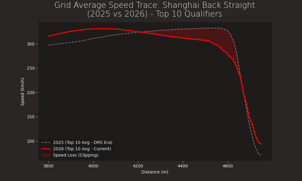
Grid Average Speed Trace: 2025 vs 2026

Compare the average speed trace of the Top 10 drivers on a long straight between two different regulation eras (2025 vs 2026). This visualization highlights the ‘clipping’ effect of the 2026 Power Units.

import matplotlib.pyplot as plt
import numpy as np
import pandas as pd

import fastf1
import fastf1.plotting

Enable FastF1’s plotting settings (dark theme etc.)

fastf1.plotting.setup_mpl(color_scheme="fastf1")

Define the session parameters. We compare the Qualifying sessions of the Chinese Grand Prix.

year_old = 2025
year_new = 2026
track = "China"
session_type = "Q"

Load the sessions.

session_old = fastf1.get_session(year_old, track, session_type)
session_new = fastf1.get_session(year_new, track, session_type)
session_old.load()
session_new.load()

Define a helper function for data interpolation. Since telemetry samples occur at different distances for each driver, we must interpolate them onto a common distance axis to calculate a mathematical average.

def get_average_speed(
    session: fastf1.core.Session, distance_array: np.ndarray
):
    """Interpolates speed for Top 10 drivers and returns the average.

    Args:
        session (fastf1.core.Session): The loaded FastF1 session
            object containing the telemetry and lap data.
        distance_array (np.ndarray): A 1D numpy array of distances
            used as the common grid for mathematical interpolation.

    Returns:
        np.ndarray: A 1D numpy array containing the calculated average
        speeds corresponding to each point in the distance_array.
    """
    speeds = []
    top_10_drivers = session.results["Abbreviation"][:10]

    for driver in top_10_drivers:
        lap = session.laps.pick_drivers(driver).pick_fastest()

        if pd.isna(lap["LapTime"]):
            continue

        tel = lap.get_telemetry().add_distance()

        # Crop telemetry to the back straight area (Shanghai)
        mask = (tel["Distance"] >= 3700) & (tel["Distance"] <= 4800)
        tel_straight = tel[mask]

        interp_speed = np.interp(
            distance_array, tel_straight["Distance"], tel_straight["Speed"]
        )
        speeds.append(interp_speed)

    return np.mean(speeds, axis=0)

Calculate the average speed traces for both years using a common distance grid.

common_distance = np.linspace(3800, 4750, 500)
avg_speed_old = get_average_speed(session_old, common_distance)
avg_speed_new = get_average_speed(session_new, common_distance)

Create the visualization. We highlight the speed delta (clipping) using a shaded area between the two traces.

fig, ax = plt.subplots(figsize=(10, 6))

ax.plot(
    common_distance,
    avg_speed_old,
    label=f"{year_old} (Top 10 Avg - DRS Era)",
    color="grey",
    linestyle="--",
)
ax.plot(
    common_distance,
    avg_speed_new,
    label=f"{year_new} (Top 10 Avg - Current)",
    color="red",
    linewidth=2.5,
)

ax.fill_between(
    common_distance,
    avg_speed_new,
    avg_speed_old,
    where=(avg_speed_old > avg_speed_new),
    color="red",
    alpha=0.2,
    label="Speed Loss (Clipping)",
)

ax.set_title(
    f"Grid Average Speed Trace: Shanghai Back Straight\n"
    f"({year_old} vs {year_new}) - Top 10 Qualifiers"
)
ax.set_xlabel("Distance (m)")
ax.set_ylabel("Speed (km/h)")
ax.legend()

plt.show()